Factor Stochastic Volatility

Factor Stochastic Volatility Model

A factor structure can be used in order to model a full time varying covariance matrix. This reduces the amount of parameters to learn; if the covariance matrix is \(p \times p\) and the number of factors used \(k\), then the number of parameters to learn in a model with an AR(1) latent-state is \(p \times k - \frac{k}{2}(k + 1) + 3k\). If \(k << p\) then this results in a much lower dimensional parameter space.

The factor stochastic volatility (FSV) model is written as:

\[\begin{align} Y_t &= \beta^Tf_t + v_t, &v_t &\sim \mathcal{N}(0, V), \\ f_t &= \sigma_t\exp\left\{ \frac{\alpha_t}{2} \right\}, & \sigma_t &\sim \mathcal{N}(0, 1), \\ \alpha_t &= \mu + \phi (\alpha_{t-1} - \mu) + \eta_t, & \eta_t &\sim \mathcal{N}(0, \sigma_\eta), \\ \alpha_0 &\sim \mathcal{N}(0, \sigma^2/(1-\phi^2)). \end{align}\]

Where \(V\) is a diagonal \(p \times p\) matrix. Then the variance of the observations is:

\[\begin{align} \operatorname{Var}(Y_t) &= \operatorname{Var}(\beta^Tf_t + v_t) \\ &= \beta^T\operatorname{Var}(f_t)\beta + \operatorname{Var}(v_t) + 2\beta^T\operatorname{Cov}(f_t, v_t)\beta \\ &= \beta^T\exp\left\{\alpha_t\right\}\beta + V \end{align}\]

To define the factor stochastic volatility model, define the parmeters of the model and simulate using the parameters:

scala> import com.github.jonnylaw.dlm._
<console>:12: warning: Unused import
       import com.github.jonnylaw.dlm._
                                      ^
import com.github.jonnylaw.dlm._

scala> import breeze.linalg.DenseMatrix
<console>:10: warning: Unused import
       import com.github.jonnylaw.dlm._
                                      ^
<console>:15: warning: Unused import
       import breeze.linalg.DenseMatrix
                            ^
import breeze.linalg.DenseMatrix

scala> val beta = DenseMatrix((1.0, 0.0),
     |                        (0.3, 1.0),
     |                        (0.07, 0.25),
     |                        (0.23, 0.23),
     |                        (0.4, 0.25),
     |                        (0.2, 0.23))
<console>:10: warning: Unused import
       import com.github.jonnylaw.dlm._
                                      ^
beta: breeze.linalg.DenseMatrix[Double] =
1.0   0.0
0.3   1.0
0.07  0.25
0.23  0.23
0.4   0.25
0.2   0.23

scala> val params = FsvParameters(
     |   v = DenseMatrix.eye[Double](6) * 0.1,
     |   beta,
     |   Vector.fill(2)(SvParameters(0.8, 2.0, 0.3))
     | )
params: com.github.jonnylaw.dlm.FsvParameters =
FsvParameters(0.1  0.0  0.0  0.0  0.0  0.0
0.0  0.1  0.0  0.0  0.0  0.0
0.0  0.0  0.1  0.0  0.0  0.0
0.0  0.0  0.0  0.1  0.0  0.0
0.0  0.0  0.0  0.0  0.1  0.0
0.0  0.0  0.0  0.0  0.0  0.1  ,1.0   0.0
0.3   1.0
0.07  0.25
0.23  0.23
0.4   0.25
0.2   0.23  ,Vector(SvParameters(0.8,2.0,0.3), SvParameters(0.8,2.0,0.3)))

scala> val sims = FactorSv.simulate(params).steps.take(1000)
<console>:12: warning: Unused import
       import breeze.linalg.DenseMatrix
                            ^
sims: Iterator[(com.github.jonnylaw.dlm.Data, scala.collection.immutable.Vector[Double], scala.collection.immutable.Vector[Double])] = <iterator>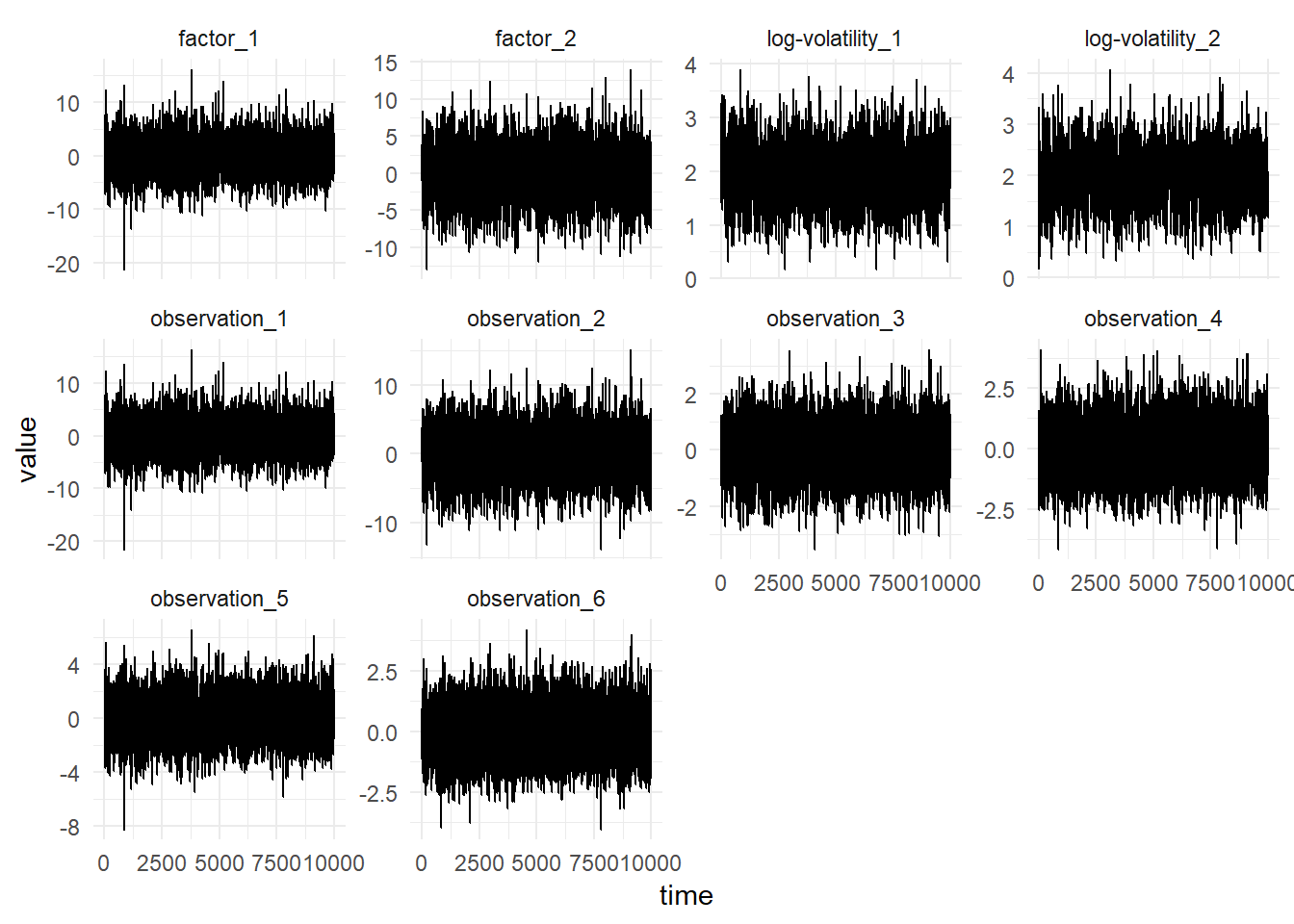

Parameter Inference

Gibbs sampling is used to perform inference for the parameter posterior distribution. First the prior distributions of the parameters can be specified, they must be from the same family as the distributions below, since the posterior distributions in Gibbs sampling are conditionally conjugate:

scala> import breeze.stats.distributions._
<console>:10: warning: Unused import
       import com.github.jonnylaw.dlm._
                                      ^
<console>:12: warning: Unused import
       import breeze.linalg.DenseMatrix
                            ^
<console>:16: warning: Unused import
       import breeze.stats.distributions._
                                         ^
import breeze.stats.distributions._

scala> val priorBeta = Gaussian(0.0, 1.0)
<console>:10: warning: Unused import
       import com.github.jonnylaw.dlm._
                                      ^
<console>:12: warning: Unused import
       import breeze.linalg.DenseMatrix
                            ^
priorBeta: breeze.stats.distributions.Gaussian = Gaussian(0.0, 1.0)

scala> val priorSigmaEta = InverseGamma(2, 2.0)
<console>:12: warning: Unused import
       import breeze.linalg.DenseMatrix
                            ^
<console>:14: warning: Unused import
       import breeze.stats.distributions._
                                         ^
priorSigmaEta: com.github.jonnylaw.dlm.InverseGamma = InverseGamma(2.0,2.0)

scala> val priorPhi = Gaussian(0.8, 0.1)
<console>:10: warning: Unused import
       import com.github.jonnylaw.dlm._
                                      ^
<console>:12: warning: Unused import
       import breeze.linalg.DenseMatrix
                            ^
priorPhi: breeze.stats.distributions.Gaussian = Gaussian(0.8, 0.1)

scala> val priorMu = Gaussian(2.0, 1.0)
<console>:10: warning: Unused import
       import com.github.jonnylaw.dlm._
                                      ^
<console>:12: warning: Unused import
       import breeze.linalg.DenseMatrix
                            ^
priorMu: breeze.stats.distributions.Gaussian = Gaussian(2.0, 1.0)

scala> val priorSigma = InverseGamma(10, 2.0)
<console>:12: warning: Unused import
       import breeze.linalg.DenseMatrix
                            ^
<console>:14: warning: Unused import
       import breeze.stats.distributions._
                                         ^
priorSigma: com.github.jonnylaw.dlm.InverseGamma = InverseGamma(10.0,2.0)

Then performing Gibbs sampling for the FSV model using the simulated data, sims:

scala> val iters = FactorSv.sampleAr(priorBeta,
     |             priorSigmaEta,
     |             priorMu,
     |             priorPhi,
     |             priorSigma,
     |             sims.toVector.map(_._1),
     |             params)
<console>:12: warning: Unused import
       import breeze.linalg.DenseMatrix
                            ^
<console>:16: warning: Unused import
       import breeze.stats.distributions._
                                         ^
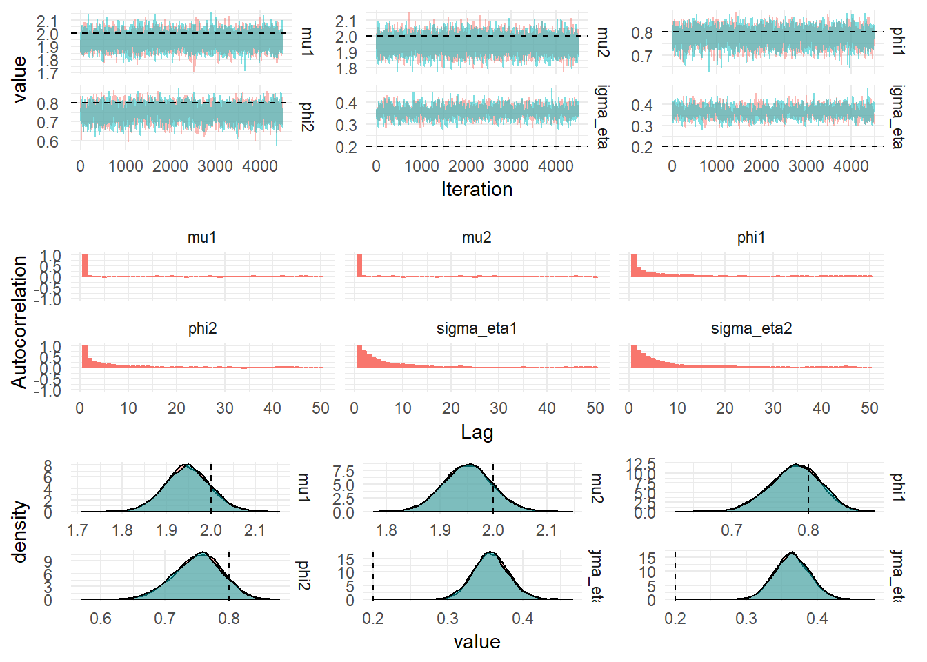
iters: breeze.stats.distributions.Process[com.github.jonnylaw.dlm.FactorSv.State] = breeze.stats.distributions.MarkovChain$$anon$1@6fbac0da

The figure below shows the diagnostics from 100,000 iterations of the MCMC with the first 10,000 iterations dropped for burn-in and every 20th iteration selected.

Parameter	mean	median	upper	lower	ESS	actual_value
beta1	1.0000000	1.0000000	1.0000000	1.0000000	NaN	1.00
beta10	0.2334747	0.2334737	0.2335777	0.2333746	2802	0.23
beta11	0.2530543	0.2530527	0.2531831	0.2529261	2913	0.25
beta12	0.2307056	0.2307050	0.2308070	0.2306065	2957	0.23
beta2	0.3136651	0.3136611	0.3140995	0.3132333	2940	0.30
beta3	0.0722864	0.0722852	0.0724226	0.0721516	2884	0.07
beta4	0.2344680	0.2344690	0.2345967	0.2343358	3038	0.23
beta5	0.4060201	0.4060203	0.4061998	0.4058379	3093	0.40
beta6	0.2039967	0.2039964	0.2041210	0.2038716	3005	0.20
beta7	0.0000000	0.0000000	0.0000000	0.0000000	NaN	0.00
beta8	1.0000000	1.0000000	1.0000000	1.0000000	NaN	1.00
beta9	0.2510994	0.2510981	0.2512251	0.2509793	2979	0.25