Stochastic Volatility
Stochastic volatility models are a class of models for non-stationary time series data. The log of the variance of the series is assumed to evolve according to a latent Gaussian process. The equation below shows a univariate stochastic volatility model with an AR(1) latent state:
\[\begin{align*} Y_t &= \varepsilon_t\exp(\alpha_t/2), &\varepsilon_t &\sim \mathcal{N}(0, 1), \\ \alpha_t &= \mu + \phi(\alpha_{t-1} - \mu) + \eta_t, &\eta_t &\sim \mathcal{N}(0, \sigma_\eta^2).\numberthis \label{eq:usv-spec} \end{align*}\]\(Y_t\), \(t = 1,\dots,T\) are discrete observations of a time series process. The latent state represents the log-volatility and \(\alpha_t\) follows an AR(1) process with mean \(\mu\).
The figure below shows a simulation from this model with fixed values of the parameters, \(\phi = 0.8, \mu = 1, \sigma_\eta = 0.1\), the initial state of the log-volatility is the stationary solution of the AR(1) process: \(\alpha_0 \sim \mathcal{N}\left(\mu, \frac{\sigma_\eta^2}{1 - \phi^2}\right)\).
To define this model in Scala and simulate observations, first import the required libraries and use the method simulate which initialises a Breeze MarkovChain object with the initial state equivalent to the stationary solution of the AR(1) process.
scala> import com.github.jonnylaw.dlm._
<console>:12: warning: Unused import
       import com.github.jonnylaw.dlm._
                                      ^
import com.github.jonnylaw.dlm._

scala> import cats.implicits._
<console>:10: warning: Unused import
       import com.github.jonnylaw.dlm._
                                      ^
<console>:15: warning: Unused import
       import cats.implicits._
                             ^
import cats.implicits._

scala> val p = SvParameters(phi = 0.8, mu = 2.0, sigmaEta = 0.3)
<console>:13: warning: Unused import
       import cats.implicits._
                             ^
p: com.github.jonnylaw.dlm.SvParameters = SvParameters(0.8,2.0,0.3)

scala> val sims = StochasticVolatility.simulate(p).
     |   steps.take(1000).toVector.tail.map { case (t, y, a) => (t, y)}
<console>:13: warning: Unused import
       import cats.implicits._
                             ^
sims: scala.collection.immutable.Vector[(Double, Option[Double])] = Vector((2.0,Some(3.846583926103539)), (3.0,Some(-0.23095146212092024)), (4.0,Some(-3.4143942394698206)), (5.0,Some(1.7572309122071414)), (6.0,Some(2.1047649586787083)), (7.0,Some(-2.2661717069966496)), (8.0,Some(0.4066468240993743)), (9.0,Some(-0.3843542564748422)), (10.0,Some(-4.271175785394365)), (11.0,Some(2.2641525966108533)), (12.0,Some(0.832053197800046)), (13.0,Some(-1.071886957638012)), (14.0,Some(-4.587727837914248)), (15.0,Some(0.4561115567367286)), (16.0,Some(0.7214564076353294)), (17.0,Some(-1.2356909193260661)), (18.0,Some(3.9836016044778764)), (19.0,Some(1.2202853102451159)), (20.0,Some(0.562178388757327)), (21.0,Some(5.0632597721313735)), (22.0,Some(-1.0518501203753887)), (23.0,Some(0.7311813047530124)), ...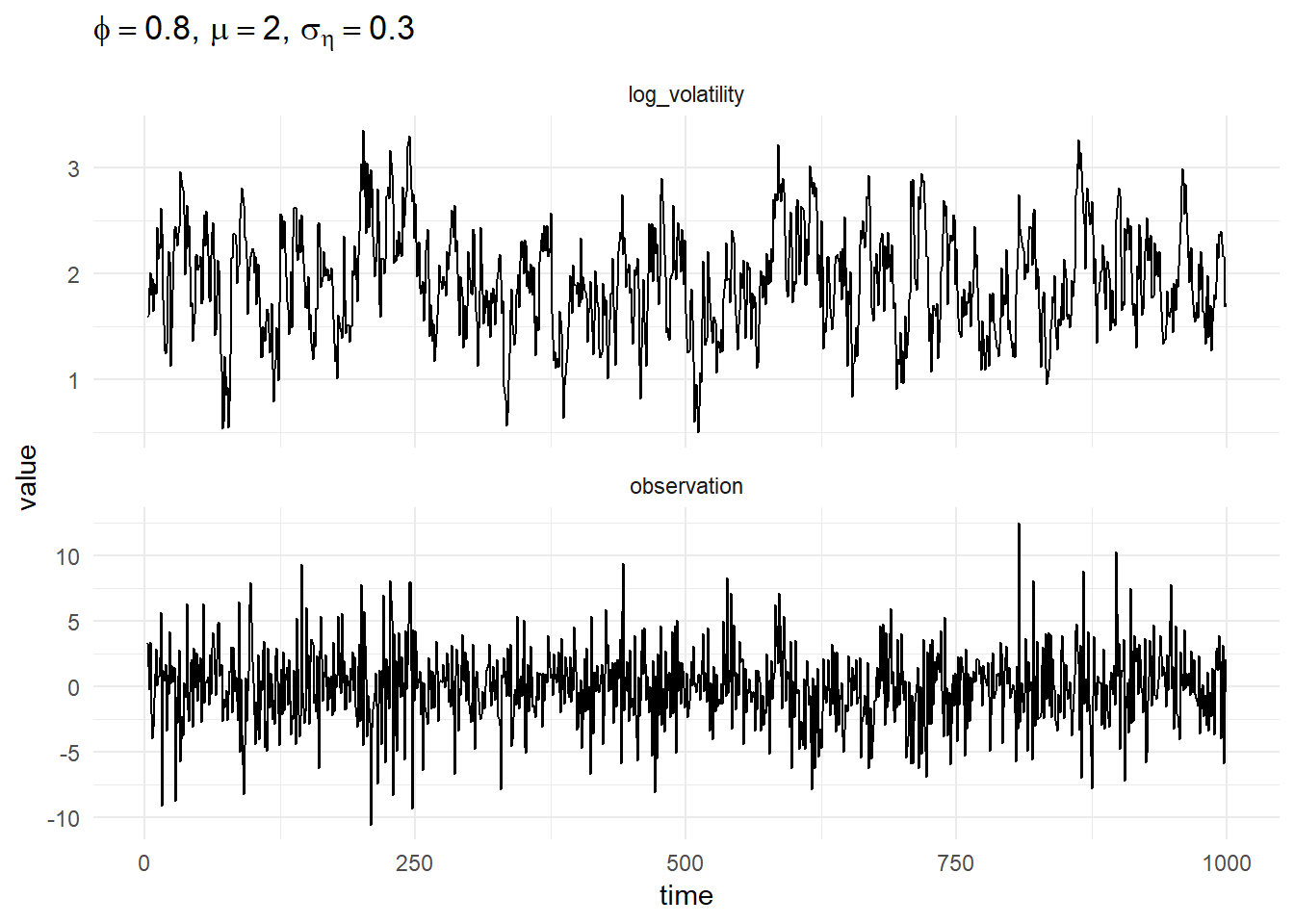
Parameter Inference
To determine the posterior distribution of the parameters specify the prior distributions of the parameters:
scala> import breeze.stats.distributions.Gaussian
<console>:10: warning: Unused import
       import com.github.jonnylaw.dlm._
                                      ^
<console>:13: warning: Unused import
       import cats.implicits._
                             ^
<console>:18: warning: Unused import
       import breeze.stats.distributions.Gaussian
                                         ^
import breeze.stats.distributions.Gaussian

scala> val priorPhi = Gaussian(0.8, 0.1)
<console>:10: warning: Unused import
       import com.github.jonnylaw.dlm._
                                      ^
<console>:13: warning: Unused import
       import cats.implicits._
                             ^
priorPhi: breeze.stats.distributions.Gaussian = Gaussian(0.8, 0.1)

scala> val priorMu = Gaussian(2.0, 1.0)
<console>:10: warning: Unused import
       import com.github.jonnylaw.dlm._
                                      ^
<console>:13: warning: Unused import
       import cats.implicits._
                             ^
priorMu: breeze.stats.distributions.Gaussian = Gaussian(2.0, 1.0)

scala> val priorSigma = InverseGamma(2.0, 2.0)
<console>:13: warning: Unused import
       import cats.implicits._
                             ^
<console>:15: warning: Unused import
       import breeze.stats.distributions.Gaussian
                                         ^
priorSigma: com.github.jonnylaw.dlm.InverseGamma = InverseGamma(2.0,2.0)
There are two inference algorithms defined for the stochastic volatility model, either one can be used and should produce identical inferences:
y1. Likelihood Analysis of Non-Gaussian Measurement Time Series: http://www.jstor.org/stable/2337586 2. Stochastic volatility: likelihood inference and comparison with ARCH models: https://faculty.mccombs.utexas.edu/carlos.carvalho/teaching/KSB98-SV.pdf
scala> val iters1 = StochasticVolatilityKnots.sampleParametersAr(priorPhi,
| priorMu,
| priorSigma,
| sims)
<console>:13: warning: Unused import
import cats.implicits._
^
<console>:16: warning: Unused import
import breeze.stats.distributions.Gaussian
^
iters1: breeze.stats.distributions.Process[com.github.jonnylaw.dlm.StochVolState] = breeze.stats.distributions.MarkovChain$$anon$1@dcf30df
scala> val iters2 = StochasticVolatility.sampleUni(priorPhi, priorMu, priorSigma, sims)
<console>:13: warning: Unused import
import cats.implicits._
^
<console>:16: warning: Unused import
import breeze.stats.distributions.Gaussian
^
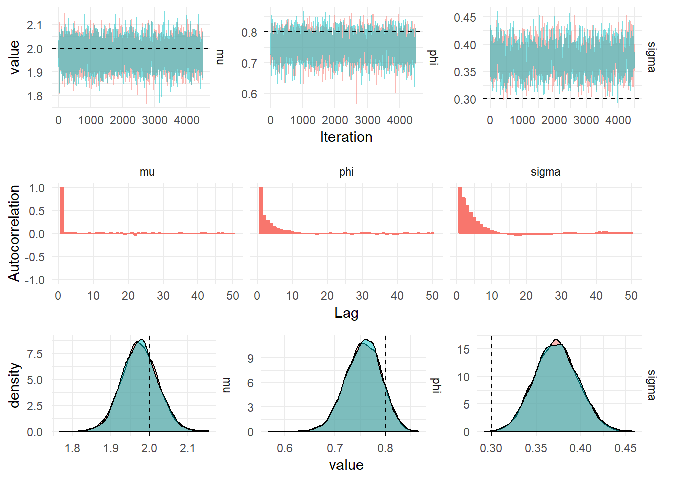
iters2: breeze.stats.distributions.Process[com.github.jonnylaw.dlm.StochVolState] = breeze.stats.distributions.MarkovChain$$anon$1@87ff76cThe figure below shows the diagnostic plots for the posterior distribution of the parameters of the univariate stochastic volatility model.