Forecasting
Forecasting using a DLM
Performing forecasting for future observations of the process using a DLM is equivalent to running the Kalman Filter without any observations in the period of the time of interest. The filter must be initialised using the posterior distribution of the latent state at the time of the last observation, \(x_T \sim \mathcal{N}(m_T, C_T)\) and the static parameters, \(\theta = (V, W)\) have been previously identified using an appropriate parameter learning technique.
Example: Seasonal Model
Define the seasonal model:
import com.github.jonnylaw.dlm._
import cats.implicits._

val mod = Dlm.polynomial(1) |+| Dlm.seasonal(24, 3)
Read in some simulated values from the seasonal model.
import breeze.linalg._
import java.nio.file.Paths
import kantan.csv._
import kantan.csv.ops._

val rawData = Paths.get("examples/data/seasonal_dlm.csv")
val reader = rawData.asCsvReader[List[Double]](rfc.withHeader)
val data = reader.
  collect {
    case Right(a) => Data(a.head.toInt, DenseVector(Some(a(1))))
  }.
  toVector
Then calculate the mean value of the MCMC parameters, assuming that the parameters have been written to a CSV called seasonal_dlm_gibbs.csv with eight columns, \(V, W_1,\dots,W_7\):
import breeze.stats.mean

val mcmcChain = Paths.get("examples/data/seasonal_dlm_gibbs.csv")
val read = mcmcChain.asCsvReader[List[Double]](rfc.withHeader)

val params: List[Double] = read.
  collect { case Right(a) => a }.
  toList.
  transpose.
  map(a => mean(a))

val meanParameters = DlmParameters(
  v =  DenseMatrix(params.head),
  w =  diag(DenseVector(params.tail.toArray)),
  m0 = DenseVector.zeros[Double](7),
  c0 = DenseMatrix.eye[Double](7)
 )
When then use these parameters to get the posterior distribution of the final state:
val filtered = KalmanFilter.filterDlm(mod, data, meanParameters)
val (mt, ct, initTime) = filtered.map(a => (a.mt, a.ct, a.time)).last
We then initialise the forecast function with state state posterior at the time of the last observation:
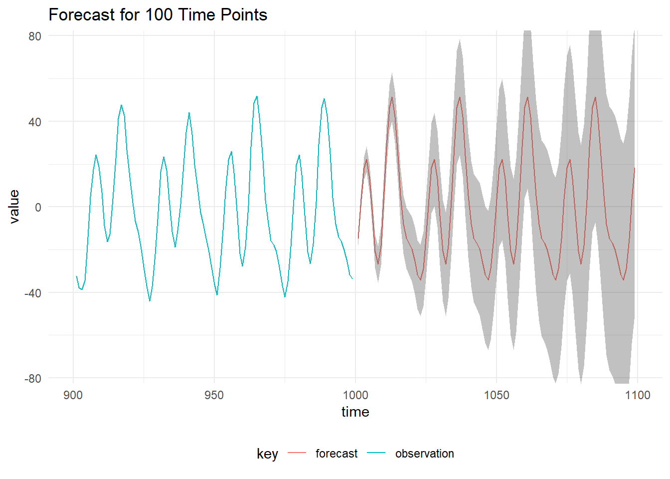
val forecasted = Dlm.forecast(mod, mt, ct, initTime, meanParameters).
  take(100).
  toList
The results of the forecasting and 95% prediction intervals are below:
Forecasting using a DGLM
The Kalman Filter can not be applied to state space models with non-Gaussian observation distributions. Particle filtering is commonly used to approximate the filtering distribution using a cloud of \(M\) particles. The time series currently has observations at times \(t = 1,\dots,T\) and we are interested in an observation \(k\) time-steps in the future:
- Obtain a sample of the latent state at the time of the final observation, \(p(x_T|y_{1:T}, x_{0:{T-1}}, \theta) = \{x_T^{(j)}, j = 1,\dots, M\}\)
- Advance the state using the model’s state evolution density, \(p(x_{T+k}^{(j)}|x_{T}^{(j)}, W)\), \(j = 1,\dots,M\)
- Draw from the observation distribution using each particle as a sample from the latent-state, \(p(y^{(j)}_{T+k}|x_{T+k}^{(j)}, V)\)
Summaries of the observation distribution can then be calculated.
Example: DGLM Forecast
TODO