Simulate Data

The data is simulated from a second order DLM:

\[\begin{align} Y_t &= F \textbf{x}_t + v_t, \quad v_t \sim \mathcal{N}(0, V), \\ \textbf{X}_t &= G \textbf{x}_{t-1} + \textbf{w}_t, \quad w_t \sim \textrm{MVN}(0, W), \\ \textbf{X}_0 &\sim \textrm{MVN}(m_0, C_0). \end{align}\]

The state is two dimensional, as such the system noise matrix \(W\) is a \(2 \times 2\) matrix. The observation and system evolution matrices do not depend on time, the observation matrix is \(F = (1 \quad 0)\) and the system evolution matrix is:

\[G = \begin{pmatrix} 1 & 1 \\ 0 & 1 \end{pmatrix}.\]

In order to examine the properties of this model, first we can simulate a time series of values from it:

import com.github.jonnylaw.dlm._
import breeze.linalg.{DenseMatrix, DenseVector, diag}

val mod = Dlm.polynomial(2)
  val p = DlmParameters(
    DenseMatrix(3.0),
    diag(DenseVector(2.0, 1.0)),
    DenseVector(0.0, 0.0),
    diag(DenseVector(100.0, 100.0))
  )

val data = Dlm.simulateRegular(mod, p, 1.0).
  steps.
  take(1000).
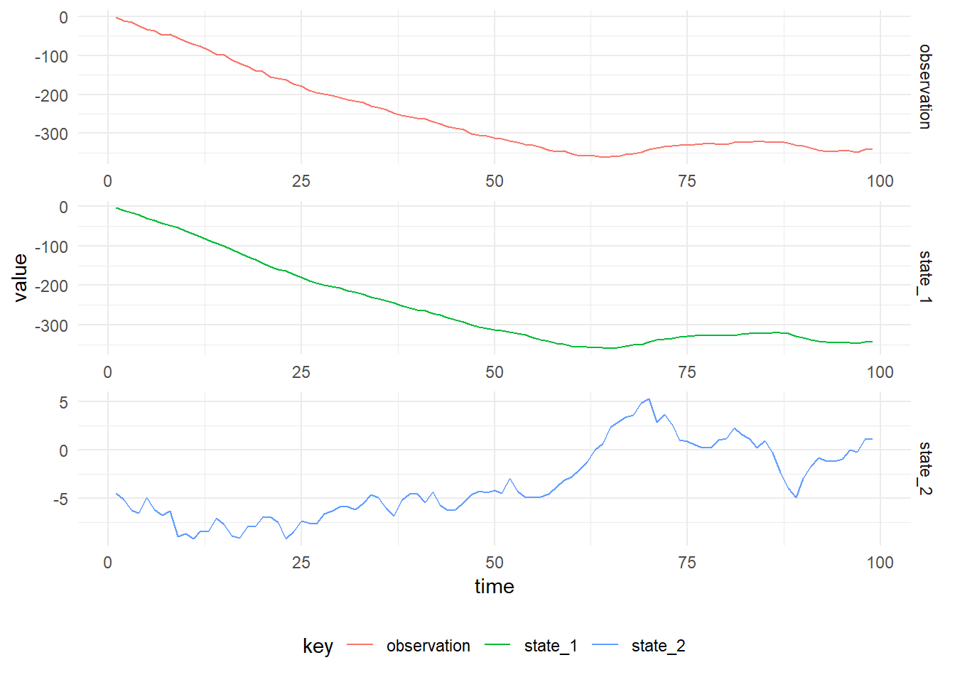
  toVector

The figure below shows simulated values from the Second Order DLM with parameters, \((V, W, \textbf{m}_0, C_0) = (3.0, \operatorname{diag}(2.0, 1.0), (0.0, 0.0), \operatorname{diag}(100.0, 100.0))\)

Filtered

Kalman Filtering can be performed to learn the posterior distribution of the states, given the observations:

import cats.implicits._
val filtered = KalmanFilter.filterDlm(mod, data.map(_._1), p)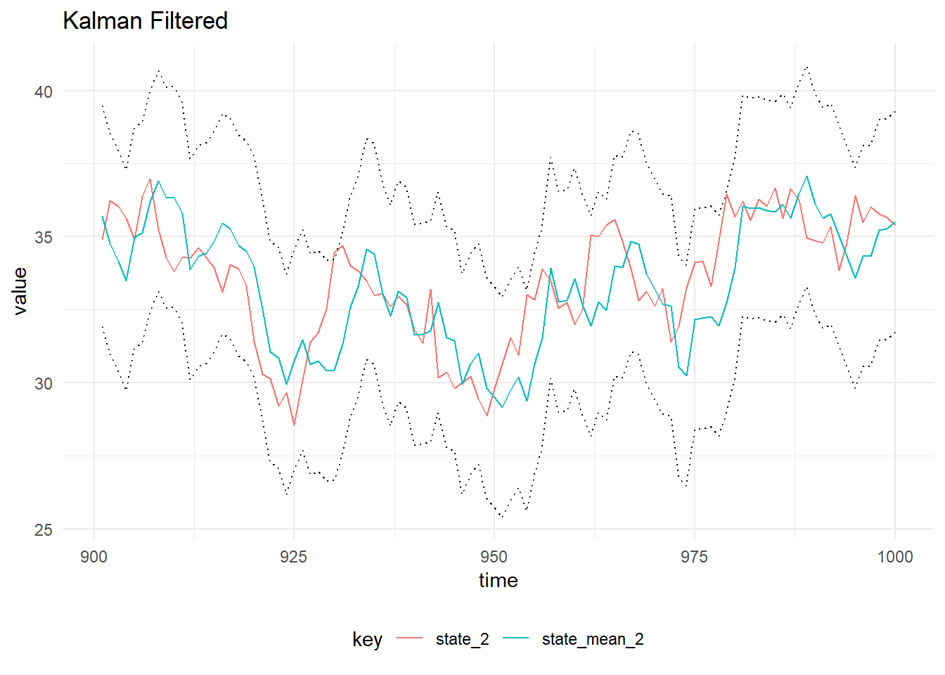

Filtered State of the second order model, with 90% probability intervals

Parameters Inference

The parameter posterior distributions can be learned using Gibbs sampling. The state evolution distribution and the observation distribution are Gaussian with unknown variance \(W\) and \(V\) respectively. The state is assumed to have a diagonal, \(2 \times 2\) covariance matrix and hence the unknown variances are chosen to have Inverse Gamma priors. The Inverse Gamma distribution is conjugate to the Normal distribution with known mean and unknown variance. To perform gibbs sampling using the Bayesian DLMs package:

val iters = GibbsSampling.sample(
    mod,
    InverseGamma(4.0, 9.0),
    InverseGamma(5.0, 8.0),
    p,
    data.map(_._1))

gibbs_iters = read_csv("../examples/data/second_order_dlm_gibbs.csv")

actual_values = tibble(
  Parameter = c("V", "W1", "W2"),
  actual_value = c(3.0, 2.0, 1.0)
)

# gibbs_iters %>%
#   mcmc() %>% ggs() %>%
#   summary_table()

params = ggs(mcmc(gibbs_iters))

p1 = params %>%
  inner_join(actual_values) %>%
  ggplot(aes(x = Iteration, y = value)) +
  geom_line() +
  geom_hline(aes(yintercept = actual_value), colour = "#ff0000") +
  facet_wrap(~Parameter, scales = "free_y")

p2 = params %>%
  ggs_autocorrelation()

p1 + p2 + plot_layout(ncol = 1)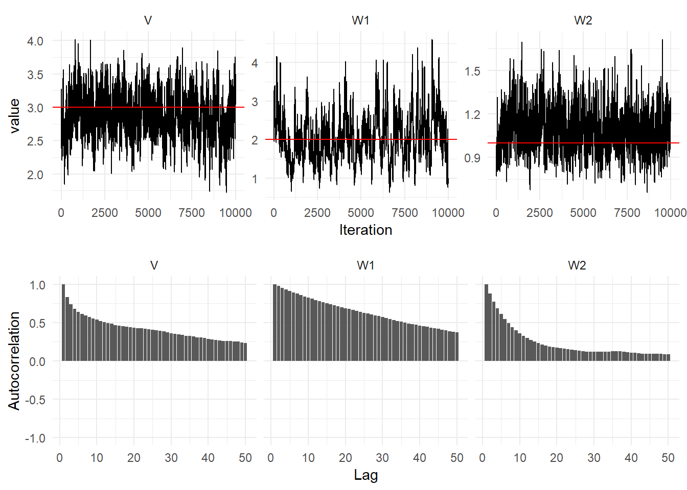

Diagnostic plots of the parameter posterior distributions for the second order DLM (Top) Traceplots (Bottom) Autocorrelation