Student’s t-distributed DLM
The Student’s t-distribution has thicker tails than the normal distribution for low values of the degrees of freedom hence is more foregiving of outliers in the measurements. The scaled, shifted Student’s t-distribution is parameterised by the location, \(\ell\), scale \(s\) and degrees of freedom \(\nu\), the probability density function is:
\[p(x|\ell, s, \nu) = \frac{\Gamma\left(\frac{\nu + 1}{2}\right)}{\sqrt{\pi\nu s}\Gamma(\frac{\nu}{2})} \left(\frac{(x-\ell)^2}{\nu s^2} + 1 \right)^{- \frac{\nu + 1}{2}}\]
Then the state-space model, with a first order polynomial latent-state evolution can be written as:
\[\begin{aligned} Y_t &\sim t_\nu(x_t, s^2), \\ x_t &= x_{t-1} + w_t, \qquad w_t \sim \mathcal{N}(0, W), \\ x_0 &\sim \mathcal{N}(m_0, C_0). \end{aligned}\]
The Student’s t model is specified in scala by first specifying a DLM model, which specifys the system and observation matrices (\(G_t\) and \(F_t\)) then specifying the observation model using the Dglm class:
import com.github.jonnylaw.dlm._

val dlm = Dlm.polynomial(1)
val mod = Dglm.studentT(3, dlm)
The code below can be used to simulate 1,000 iterations from the Student’s t model.
import breeze.linalg.{DenseVector, DenseMatrix}
val params = DlmParameters(
DenseMatrix(3.0),
DenseMatrix(0.1),
DenseVector(0.0),
DenseMatrix(1.0))
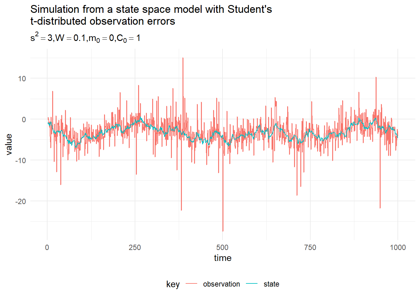
val data = Dglm.simulateRegular(mod, params, 1.0).
steps.
take(1000).
toVectorA simulation from the model with \(\{s^2, W, m_0, C_0\} = \{3, 0.1, 0, 1\}\) is presented in the figure below:
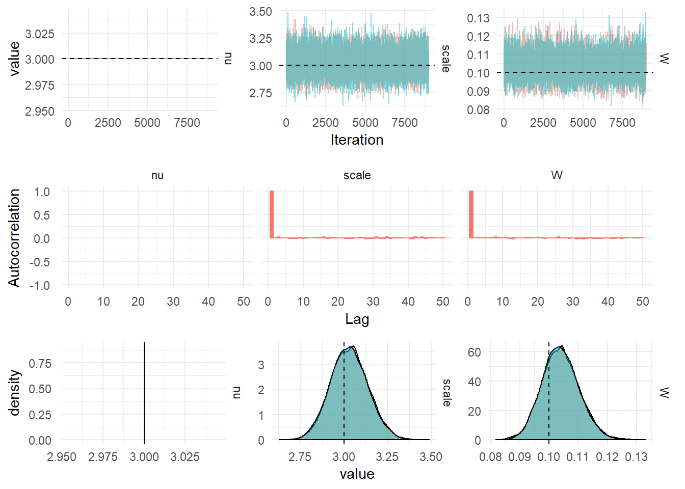
Parameter Inference
In order to fit the t-distributed state space model to observed data we need to learn the values of the parameters \(\psi = \{s^2, W, m_0, C_0\}\). A particle filter can be used to find an (unbiased) estimate of the likelihood, then Metropolis Hastings can be used to learn the posterior distribution of the parameters.
Kalman Filtering
Student’s t-distribution arises as a Inverse Gamma mixture of Normals, consider \(X | V \sim \mathcal{N}(\mu, V)\), \(W \sim \textrm{Inverse-Gamma}(\alpha, \beta)\) then the marginal distribution of \(X\) is:
\[\begin{aligned} p(X) &= \int_0^\infty p(X|V)p(V) \textrm{d}V, \\ &= \int_0^\infty \frac{\beta^\alpha}{\sqrt{2\pi}\Gamma(\alpha)} V^{-\frac{1}{2}} \exp \left(\frac{-(x-\mu)^2}{2V}\right) V^{-\alpha-1} \exp \left( -\frac{\beta}{V} \right) \textrm{d}V, \\ &= \frac{\beta^\alpha}{\sqrt{2\pi}\Gamma(\alpha)}\int_0^\infty V^{-(\alpha + \frac{1}{2}) - 1} \exp \left\{-\frac{1}{V}\left(\frac{(x-\mu)^2}{2} + \beta \right)\right\} \textrm{d}V,\\ &= \frac{\beta^\alpha\Gamma\left(\alpha + \frac{1}{2}\right)}{\sqrt{2\pi}\Gamma(\alpha)\left(\frac{(x-\mu)^2}{2} + \beta \right)^{\alpha + \frac{1}{2}} } \\ &= \frac{\beta^\alpha\Gamma\left(\alpha + \frac{1}{2}\right)}{\sqrt{2\pi}\Gamma(\alpha)\beta^{\alpha + \frac{1}{2}}\left(\frac{(x-\mu)^2}{2\beta} + 1 \right)^{\alpha + \frac{1}{2}}} \\ &= \frac{\Gamma\left(\frac{2\alpha + 1}{2}\right)}{\sqrt{2\pi\beta}\Gamma(\alpha)} \left(\frac{(x-\mu)^2}{2\beta} + 1 \right)^{- \frac{2\alpha + 1}{2}} \end{aligned}\]
Then comparing this result with the PDF of the scaled, shifted Student’s t-distribution we can see that, \(\nu = 2\alpha\), \(\ell = \mu\) and \(s = \sqrt{\beta/\alpha}\).
This derivation means we have found a way to simulate from a scaled, shifted Student’s t-distribution, by first simulating \(V_i\) from the Inverse Gamma distribution with parameters \(\alpha = \nu/2\) and \(\beta = \nu s^2/2\), then simulating from a Normal distribution with mean \(\ell\) and variance \(V_i\). Further, this means we can use Kalman Filtering for a model with a Student-t observation distribution.
Exact Filtering for the Student’s t-distribution Model
A Dynamic linear model with Student’s t-Distribution observation noise can be written as:
\[\begin{aligned} Y_t | \textbf{x}_t &\sim t_\nu(F_t \textbf{x}_t, s),\\ \textbf{X}_t | \textbf{x}_{t-1} &= G_t\textbf{x}_{t-1} + \textbf{w}_t, &\textbf{w}_t &\sim \textrm{MVN}(0, W t),\\ \textbf{X}_0 &\sim \textrm{MVN}(m_0, C_0). \end{aligned}\]
Where the location of the Student’s t-distribution is \(F_t\textbf{x}_t\), the scale and degrees of freedom are static and can be learned from the data. Consider the measurement update step of the Kalman filter with the new observation distribution:
\[p(Y_t|\textbf{x}_t) = \int_0^\infty \mathcal{N}\left(Y_t; F_t\textbf{x}_t, V_t\right)\textrm{InverseGamma}\left(V_t;\frac{\nu}{2}, \frac{\nu s^2}{2}\right) \textrm{d}V_t\]
Using the result in the previous section, that the Student’s t-distribution is an Inverse Gamma mixture of Normals. The joint distribution of all the random variables in the model can be written as:
\[\begin{aligned} p(\textbf{x}_{0:T}, y_{1:T}, s, W) &= p(W)p(x_0)\prod_{t=1}^Tp(V_t)p(Y_t|\textbf{x}_t, V_t)p(\textbf{x}_t|\textbf{x}_{t-1}, W) \\ &= \textrm{InverseGamma}(W_j; \alpha, \beta) \mathcal{N}(\textbf{x}_0; m_0, C_0)\times\\ &\prod_{t=1}^T\textrm{InverseGamma}\left(V_t; \frac{\nu}{2}, \frac{\nu s^2}{2}\right)\mathcal{N}(Y_t; F_t\textbf{x}_t, V_t)\mathcal{N}(\textbf{x}_t; G_t\textbf{x}_{t-1}, W) \end{aligned}\]
Using the Markovian property of the latent-state and the conditional independence in the model. Construct a Gibbs Sampler, the state can be sampled conditional on the observed data \(y_{1:T}\) and the parameters \(W\) and \(V_t\) using FFBS.
For the system noise matrix, assume the matrix is diagonal, with each diagonal element indexed by \(j\):
\[\begin{aligned} p(W_j|\textbf{x}_{0:T}, y_{1:T}, s, V) &= p(W)\prod_{t=1}^Tp(\textbf{x}_t|\textbf{x}_{t-1}, W) \\ &= \textrm{InverseGamma}(\alpha, \beta)\prod_{t=1}^T\mathcal{N}(G_t\textbf{x}_{t-1}, W) \\ &= \textrm{InverseGamma}\left(\alpha + \frac{T}{2}, \beta + \frac{1}{2}\sum_{i=1}^t (\textbf{x}_t - G_t\textbf{x}_{t-1})_j^2 \right). \end{aligned}\]
For the auxiliary variable, \(V_t\), the variance of the Normal distribution:
\[\begin{aligned} p(V|\textbf{x}_{0:T}, y_{1:T}, W, s) &= \prod_{t=1}^Tp(Y_t|\textbf{x}_t, V_t)p(V_t) \\ &= \prod_{t=1}^T\textrm{InverseGamma}\left(\frac{\nu}{2}, \frac{\nu s^2}{2}\right)\mathcal{N}(F_t\textbf{x}_t, V_t) \end{aligned}\]
Then for each observation of the process, we have to sample a value of the variance from:
\[\begin{aligned} p(V_t|\textbf{x}_{0:T}, y_{1:T}, W, s) &= p(Y_t|\textbf{x}_t, V_t)p(V_t), \\ &= \textrm{InverseGamma}\left(\frac{\nu + 1}{2}, \frac{\nu s^2 + (y_t - F_t\textbf{x}_t)^2}{2}\right). \end{aligned}\]
For the scale of the Student’s t-distribution, \(s^2\):
\[\begin{aligned} p(s^2|y_{1:T}, \textbf{x}_{0:T}, W, V) &= \prod_{t=1}^T\textrm{InverseGamma}\left(V_t; \frac{\nu}{2}, \frac{\nu s^2}{2}\right) \\ &\propto \prod_{t=1}^T \left(\frac{\nu s^2}{2}\right)^{\frac{\nu}{2}} \exp\left(-\frac{\nu s^2}{2V_t}\right) \\ &= \left(\frac{\nu s^2}{2}\right)^{\frac{T\nu}{2}}\exp\left(-\frac{\nu}{2} \sum_{i=1}^T\frac{s^2}{V_t}\right) \\ &\propto (s^2)^{T\nu/2}\exp\left(-\frac{\nu}{2} \sum_{i=1}^T\frac{s^2}{V_t}\right) \\ &\propto \textrm{Gamma}\left(\frac{T\nu}{2} + 1, \frac{\nu}{2} \sum_{i=1}^T\frac{1}{V_t}\right) \end{aligned}\]
Note that we have assumed the degrees of freedom of the Student’s t-distribution (\(\nu\)) is known a-priori. This can also be learned from the data using a Metropolis-Hastings step.
The Kalman Filter needs to incorporate the change of variance at each timestep. The step which has to be changed is the one-step prediction, once we have sampled the variances, \(V_t\) for each observation from the posterior distribution derived above, we can perform the Kalman filter conditional upon knowing these variances:
\[\begin{aligned} \textrm{Prediction:} & & \textrm{draw } V_t &\sim \textrm{InverseGamma}\left(\frac{\nu + 1}{2}, \frac{\nu s^2 + (y_t - F_t\textbf{x}_t)^2}{2}\right). \\ & & f_t &= F(t) a_t \\ & & Q_t &= F_t R_t F_t^\prime + V_t \end{aligned}\]
This is sufficient to learn the parameters of a DGLM with a Student’s t-Distributed observation noise. The advantage to this approach is that we don’t have the computational complexity of using a Particle Filter for each iteration of the MCMC.
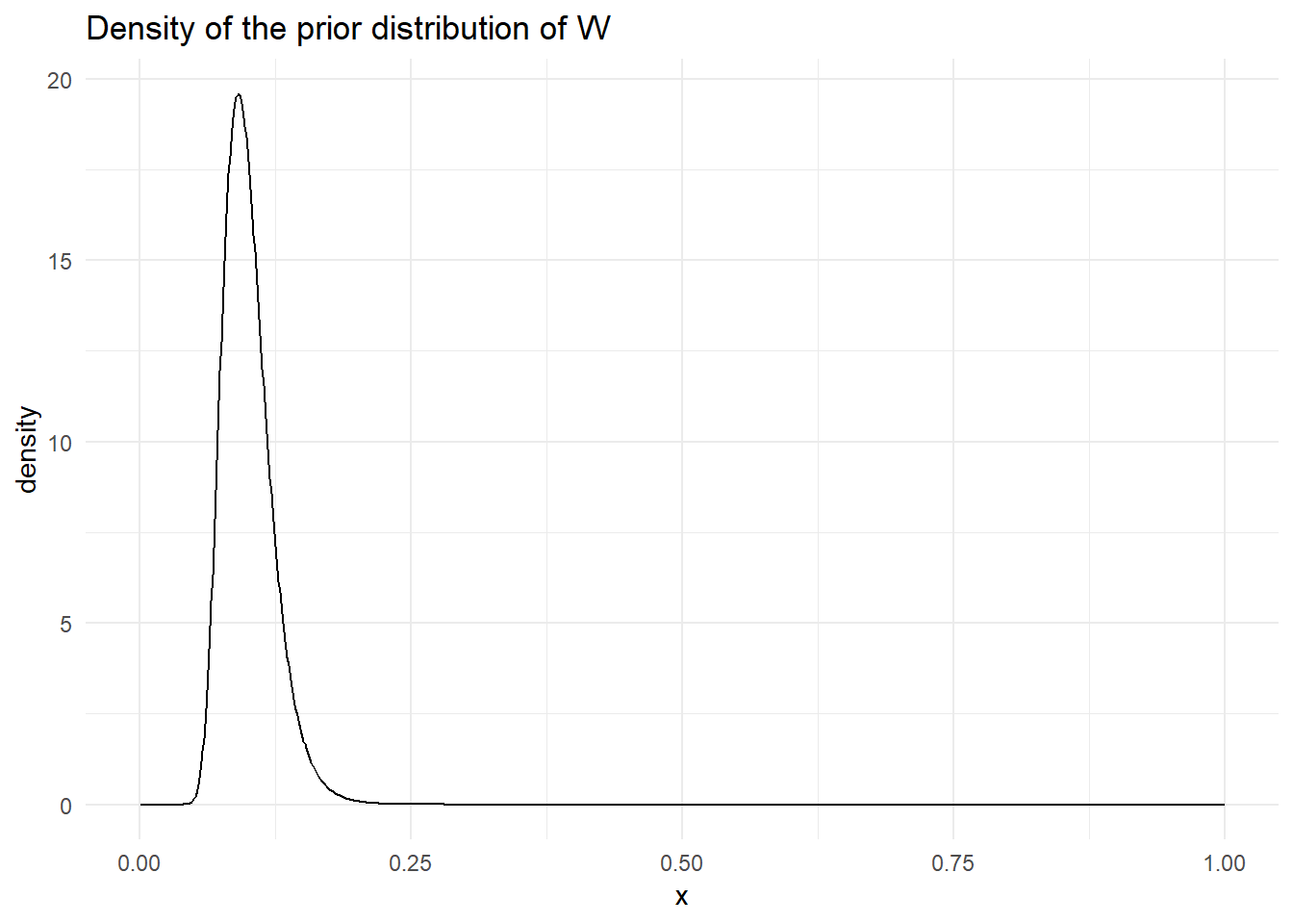
The prior distribution of the system evolution matrix is Inv-Gamma\((21, 2)\), for a mean of 0.1 and variance 0.19. The prior distribution for \(W\) looks like:
In order to run the perform Gibbs sampling on the sampled data, we use the following code:
import breeze.stats.distributions.Poisson
val propNu = (x: Int) => Poisson(x)
val propNuP = (from: Int, to: Int) => Poisson(from).logProbabilityOf(to)
val iters = StudentT.sample(data.map(_._1), InverseGamma(21.0, 2.0),
    Poisson(3), propNu, propNuP, mod, params)